Train, Optimize, Analyze, Visualize and Deploy Models for Automatic Speech Recognition with NVIDIA's NeMo
Automatic Speech Recognition (ASR) refers to automatically transcribing spoken language, otherwise known as speech-to-text. In this blog, you will learn how to use NVIDIA’s Neural Modules (NeMo) toolkit to train an end-to-end ASR system and Weights & Biases to keep track of various experiments and performance metrics.
Created on March 23|Last edited on May 20
Comment
Table of Contents (click to expand)
Introduction
In this report, we'll be looking at an Automated Speech Recognition (ASR) example using Nvidia NeMo and also showcase how to use Weights and Biases to keep track of various experiments and performance metrics.
We'll start by briefly explaining what NeMo and W&B are, along with a quick introduction to ASR generally. If you'd like to skip directly to setting up your environment, just click here.
What is Nvidia NeMo?
NVIDIA NeMo is a conversational AI toolkit built for researchers working on automatic speech recognition (ASR), natural language processing (NLP), and text-to-speech synthesis (TTS). The primary objective of NeMo is to help researchers from industry and academia to reuse prior work (code and pretrained models) and make it easier to create new conversational AI models.
What is Weights and Biases?
Weights & Biases helps machine learning teams build better models faster. With just a few lines of code, practitioners can instantly debug, compare, and reproduce their models–architecture, hyperparameters, git commits, model weights, GPU usage, datasets, and predictions–all while collaborating with their teammates.
W&B is trusted by more than 200,000 machine learning practitioners from some of the most innovative companies & research organizations in the world. It's free to get started and you can integrate in five minutes with just a couple lines of code. Click here to get started for free.
Introduction: What is Automated Speech Recognition (ASR)?
ASR, or Automatic Speech Recognition, refers to the problem of getting a program to automatically transcribe spoken language. You might know it as speech-to-text.
Our goal is usually to have a model that minimizes the Word Error Rate (WER) metric when transcribing speech input. In other words, given some audio file (e.g. a WAV file) containing speech, how do we transform this into corresponding text with as few errors as possible?
An approach like traditional speech recognition takes a generative approach, modeling the full pipeline of how speech sounds are produced in order to evaluate a speech sample. We would start from a language model that encapsulates the most likely orderings of words that are generated (e.g. an n-gram model), and incorporate a pronunciation model for each word in that ordering (e.g. a pronunciation table), as well as an acoustic model that translates those pronunciations to audio waveforms (e.g. a Gaussian Mixture Model).
Then, if we receive some spoken input, our goal would be to find the most likely sequence of text that would result in the given audio according to our generative pipeline of models. Overall, with traditional speech recognition, we try to model Pr(audio|transcript)*Pr(transcript), and take the argmax of this over possible transcripts.
Over time, neural nets advanced to the point where each component of the traditional speech recognition model could be replaced by a neural model that had better performance and that had a greater potential for generalization. The problem is that each of these neural models need to be trained individually on different tasks, and errors in any model in the pipeline could throw off the whole prediction.
Thus, we can see the appeal of end-to-end ASR architectures: discriminative models that simply take an audio input and give a textual output, and in which all components of the architecture are trained together towards the same goal. The model's encoder would be akin to an acoustic model for extracting speech features, which can then be directly piped to a decoder which outputs text. If desired, we could integrate a language model that would improve our predictions, as well.
And this way, the entire end-to-end ASR model can be trained at once--a much easier pipeline to handle!
For our task today, we'll be using Nvidia's NeMo toolkit to train an end-to-end ASR architecture and use Weights and Biases for logging performance metrics.
Let's get started!
Setting up the Environment
Now that we have some idea about Automated Speech Recognition and the tools that we're going to use as part of this blog post, the first step is to set up the environment so we can run code.
We'll first launch an instance using AWS and then install the required dependencies for NeMo to run on the machine. We'll be using Nvidia NGC and Jupyter Notebooks here.
- SSH into AWS instance and port forward 8888.
- Pull Nvidia NeMo docker container from NGC docker pull nvcr.io/nvidia/nemo:1.6.1.
- Run docker container using command docker run --runtime=nvidia -it --rm --shm-size=16g -p 8888:8888 --ulimit memlock=-1 --ulimit stack=67108864 -v $(pwd):/notebooks nvcr.io/nvidia/nemo:1.6.1.
- When inside docker container, launch Jupyter Notebook - jupyter notebook --port 8888.
- Go to localhost:8888 to access Jupyter Notebook.
- Upload downloaded files.zip in step-3 and unzip to get access to ASR W&B notebook.
And that's it! With 6 simple steps we should be inside an AWS instance with NeMo code ready to be run.
Introduction: End-to-End Automatic Speech Recognition
From the introduction to ASR section we know that it is much more helpful to be able to build an end-to-end ASR model.
With an end-to-end model, we want to directly learn Pr(transcript|audio) in order to predict the transcripts from the original audio. Since we are dealing with sequential information--audio data over time that corresponds to a sequence of letters--RNNs are an obvious choice.
But now we have a pressing problem to deal with: since our input sequence (number of audio timesteps) is not the same length as our desired output (transcript length), how do we match each time step from the audio data to the correct output characters?
Sequence-to-Sequence with Attention
A popular solution is to use a sequence-to-sequence model with attention.
A typical seq2seq model for ASR consists of some sort of bidirectional RNN encoder that consumes the audio sequence timestep-by-timestep, and where the outputs are then passed to an attention-based decoder. Each prediction from the decoder is based on attending to some parts of the entire encoded input, as well as the previously outputted tokens.
The outputs of the decoder can be anything from word pieces to phonemes to letters, and since predictions are not directly tied to time steps of the input, we can just continue producing tokens one-by-one until an end token is given (or we reach a specified max output length). This way, we do not need to deal with audio alignment, and our predicted transcript is just the sequence of outputs given by our decoder!
Taking a look at our data
If you're not familiar, AN4 consists of recordings of people spelling out addresses, names, telephone numbers, etc., one letter or number at a time, as well as their corresponding transcripts. AN4 is relatively small, with 948 training and 130 test utterances, so it trains quickly and is a great dataset for a short tutorial.
Alright, so let's download and prepare the dataset! The utterances are available as .sph format files, so we will need to convert them to .wav for processing. Run this:
# Download the datasetprint("******")if not os.path.exists(data_dir + '/an4_sphere.tar.gz'):an4_url = 'http://www.speech.cs.cmu.edu/databases/an4/an4_sphere.tar.gz'an4_path = wget.download(an4_url, data_dir)print(f"Dataset downloaded at: {an4_path}")else:print(f"Tarfile already exists at {data_dir + '/an4_sphere.tar.gz'}")an4_path = data_dir + '/an4_sphere.tar.gz'# convert .sph to .wavif not os.path.exists(data_dir + '/an4/'):# Untar and convert .sph to .wav (using sox)tar = tarfile.open(an4_path)tar.extractall(path=data_dir)sph_list = glob.glob(data_dir + '/an4/**/*.sph', recursive=True)for sph_path in tqdm(sph_list):wav_path = sph_path[:-4] + '.wav'cmd = ["sox", sph_path, wav_path]subprocess.run(cmd)
At this point, you should now have a folder called an4 that contains etc/an4_train.transcription, etc/an4_test.transcription, audio files in wav/an4_clstk and wav/an4test_clstk, along with some other files we will not need.
Let's just start with a sample audio and plot the waveform. As an example, file cen2-mgah-b.wav is a 2.6 second-long audio recording of a man saying the letters "G L E N N" one-by-one. To confirm this, we can listen to the file and plot the waveform:
import librosaimport IPython.display as ipd# Load and listen to the audio fileexample_file = data_dir + '/an4/wav/an4_clstk/mgah/cen2-mgah-b.wav'audio, sample_rate = librosa.load(example_file)ipd.Audio(example_file, rate=sample_rate)_ = librosa.display.waveplot(audio)

You can kind of tell that each spoken letter has a different "shape," and it's interesting to note that last two blobs look relatively similar, which is expected because they are both the letter "N."
Spectrograms and Mel Spectrograms
However, since audio information is more useful in the context of frequencies of sound over time, we can get a better representation if we apply a Fourier Transform on our audio signal to get something more useful: a spectrogram, which is a representation of the energy levels (i.e. amplitude, or "loudness") of each frequency (i.e. pitch) of the signal over the duration of the file.
Let's examine what the spectrogram of our sample looks like.

Again, we are able to see each letter being pronounced, and that the last two blobs that correspond to the "N"s are pretty similar-looking. But how do we interpret these shapes and colors?
Just as in the waveform plot before, we see time passing on the x-axis (all 2.6s of audio). But now, the y-axis represents different frequencies (on a log scale), and the colour on the plot shows the strength of a frequency at a particular point in time.
We're still not done yet, as we can make one more potentially useful tweak: using the Mel Spectrogram instead of the normal spectrogram. This is simply a change in the frequency scale that we use from linear (or logarithmic) to the mel scale, which is "a perceptual scale of pitches judged by listeners to be equal in distance from one another."
In other words, it's a transformation of the frequencies to be more aligned to what humans perceive; a change of +1000Hz from 2000Hz to 3000Hz sounds like a larger difference to us than 9000Hz to 10000Hz does, so the mel scale normalizes this such that equal distances sound like equal differences to the human ear.
# Plot the mel spectrogram of our samplemel_spec = librosa.feature.melspectrogram(audio, sr=sample_rate)mel_spec_db = librosa.power_to_db(mel_spec, ref=np.max)librosa.display.specshow(mel_spec_db, x_axis='time', y_axis='mel')plt.colorbar()plt.title('Mel Spectrogram');

Convolutional ASR Models
Let's take a look at the model that we will be building and how we'll specify its parameters.
The Jasper Model
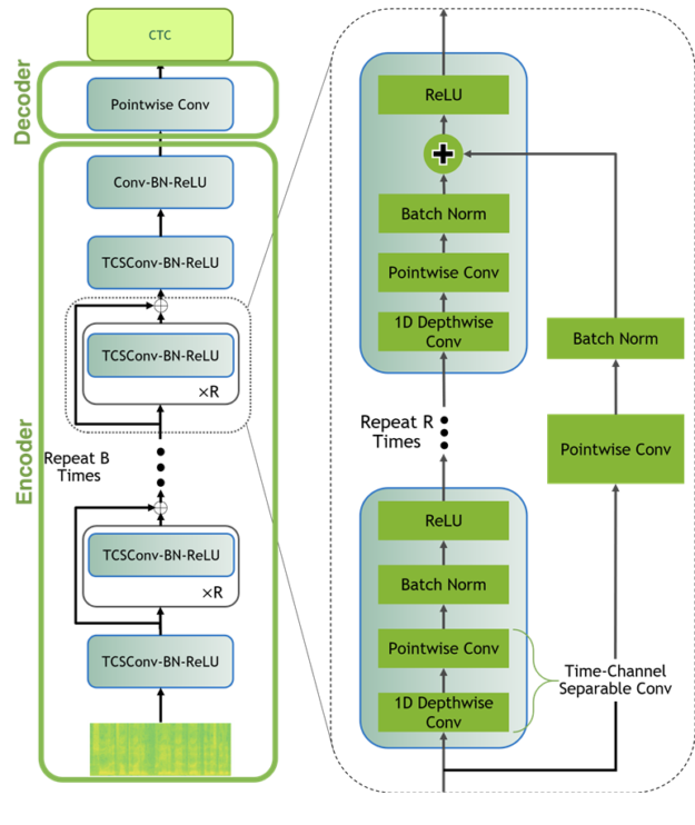
We will be training a small Jasper (Just Another SPeech Recognizer) model from scratch (e.g. initialized randomly). In brief, Jasper architectures consist of a repeated block structure that utilizes 1D convolutions. In a Jasper_KxR model, R sub-blocks (consisting of a 1D convolution, batch norm, ReLU, and dropout) are grouped into a single block, which is then repeated K times.
We also have a one extra block at the beginning and a few more at the end that are invariant of K and R, and we use CTC loss.
The QuartzNet Model
The QuartzNet is better variant of Jasper with a key difference that it uses time-channel separable 1D convolutions. This allows it to dramatically reduce number of weights while keeping similar accuracy.
A Jasper/QuartzNet models look like this (QuartzNet model is pictured):
Using NeMo for Automatic Speech Recognition
Now that we have an idea of what ASR is and how the audio data looks like, we can start using NeMo to do some ASR!
We'll be using the Neural Modules (NeMo) toolkit for this part, so if you haven't already, you should download and install NeMo and its dependencies. To do so, just follow the directions on the GitHub page, or in the documentation.
NeMo lets us easily hook together the components (modules) of our model, such as the data layer, intermediate layers, and various losses, without worrying too much about implementation details of individual parts or connections between modules. NeMo also comes with complete models which only require your data and hyperparameters for training.
# NeMo's "core" packageimport nemo# NeMo's ASR collection - this collections contains complete ASR models and# building blocks (modules) for ASRimport nemo.collections.asr as nemo_asr# This line will download pre-trained QuartzNet15x5 model from NVIDIA's NGC cloud and instantiate it for youquartznet = nemo_asr.models.EncDecCTCModel.from_pretrained(model_name="QuartzNet15x5Base-En")#
Using an Out-of-the-Box Model
NeMo's ASR collection comes with many building blocks and even complete models that we can use for training and evaluation. Moreover, several models come with pre-trained weights. Let's instantiate a complete QuartzNet15x5 model.
Next, we'll simply add paths to files we want to transcribe into the list and pass it to our model. Note that it will work for relatively short (<25 seconds) files.
files = ['./an4/wav/an4_clstk/mgah/cen2-mgah-b.wav']for fname, transcription in zip(files, quartznet.transcribe(paths2audio_files=files)):print(f"Audio in {fname} was recognized as: {transcription}")
That was easy! But there are plenty of scenarios where you would want to fine-tune the model on your own data or even train from scratch. For example, this out-of-the box model will obviously not work for Spanish and would likely perform poorly for telephone audio. So if you have collected your own data, you certainly should attempt to fine-tune or train on it!
Training from scratch
To train from scratch, you need to prepare your training data in the right format and specify your models architecture.
Creating Data Manifests from Scratch
If we were to train a model from scratch, we would have to setup our data in the right format. Therefore we need to create manifests for our training and evaluation data, which will contain the metadata of our audio files. NeMo data sets take in a standardized manifest format where each line corresponds to one sample of audio, such that the number of lines in a manifest is equal to the number of samples that are represented by that manifest. A line must contain the path to an audio file, the corresponding transcript (or path to a transcript file), and the duration of the audio sample.
Here's an example of what one line in a NeMo-compatible manifest might look like:
{"audio_filepath": "path/to/audio.wav", "duration": 3.45, "text": "this is a nemo tutorial"}
We can build our training and evaluation manifests using an4/etc/an4_train.transcription and an4/etc/an4_test.transcription, which have lines containing transcripts and their corresponding audio file IDs:
...<s> P I T T S B U R G H </s> (cen5-fash-b)<s> TWO SIX EIGHT FOUR FOUR ONE EIGHT </s> (cen7-fash-b)...
# Function to build a manifestdef build_manifest(transcripts_path, manifest_path, wav_path):audio_paths=[]; durations=[]; texts=[]with open(transcripts_path, 'r') as fin:with open(manifest_path, 'w') as fout:for line in fin:# Lines look like this:# <s> transcript </s> (fileID)transcript = line[: line.find('(')-1].lower()transcript = transcript.replace('<s>', '').replace('</s>', '')transcript = transcript.strip()file_id = line[line.find('(')+1 : -2] # e.g. "cen4-fash-b"audio_path = os.path.join(data_dir, wav_path,file_id[file_id.find('-')+1 : file_id.rfind('-')],file_id + '.wav')duration = librosa.core.get_duration(filename=audio_path)audio_paths.append(audio_path)durations.append(duration)texts.append(transcript)# Write the metadata to the manifestmetadata = {"audio_filepath": audio_path,"duration": duration,"text": transcript}json.dump(metadata, fout)fout.write('\n')return audio_paths, durations, texts# Building Manifeststrain_transcripts = data_dir + '/an4/etc/an4_train.transcription'train_manifest = data_dir + '/an4/train_manifest.json'train_audio_paths, train_durations, train_texts = build_manifest(train_transcripts, train_manifest, 'an4/wav/an4_clstk')test_transcripts = data_dir + '/an4/etc/an4_test.transcription'test_manifest = data_dir + '/an4/test_manifest.json'test_audio_paths, test_durations, test_texts = build_manifest(test_transcripts, test_manifest, 'an4/wav/an4test_clstk')
Now, once we have the train and test manifests ready, let's see how they look like!
The first five rows of the train_manifest look like this: (You can easily see for yourself with this command - !head {train_manifest} -n5)
{"audio_filepath": "./an4/wav/an4_clstk/fash/an251-fash-b.wav", "duration": 1.0, "text": "yes"}{"audio_filepath": "./an4/wav/an4_clstk/fash/an253-fash-b.wav", "duration": 0.7, "text": "go"}{"audio_filepath": "./an4/wav/an4_clstk/fash/an254-fash-b.wav", "duration": 0.9, "text": "yes"}{"audio_filepath": "./an4/wav/an4_clstk/fash/an255-fash-b.wav", "duration": 2.6, "text": "u m n y h six"}{"audio_filepath": "./an4/wav/an4_clstk/fash/cen1-fash-b.wav", "duration": 3.5, "text": "h i n i c h"}
Logging Data to Weights and Biases Table
Now that we have the data manifests ready, don't you think it will be helpful to be able to play around with the data? Maybe have the data path, audio, spectogram and mel spectogram all in one place?
Did you know it's possible to log any kind of media using Weights and Biases tables? Let me show you how.
First, we go through every audio_filepath and save a spectogram and mel-spectogram image for the audio file. Next, we create a wandb.Table to log the file name, audio file, text (the target for our model), spectogram image & mel spectogram image.
You can find the code to be able to do this below:
def save_spectogram_as_img(audio_path, datadir, plt_type='spec'):filename = os.path.basename(audio_path)out_path = os.path.join(datadir, filename.replace('.wav', '.png'))audio, sample_rate = librosa.load(audio_path)if plt_type=='spec':spec = np.abs(librosa.stft(audio))spec_db = librosa.amplitude_to_db(spec, ref=np.max)else:mel_spec = librosa.feature.melspectrogram(audio, sr=sample_rate)mel_spec_db = librosa.power_to_db(mel_spec, ref=np.max)fig = plt.Figure()ax = fig.add_subplot()ax.set_axis_off()librosa.display.specshow(spec_db if plt_type=='spec' else mel_spec_db,y_axis='log' if plt_type=='spec' else 'mel',x_axis='time', ax=ax)fig.savefig(out_path)# convert audio file to spectogram and mel spectogram imagesif not os.path.exists('./an4/melspectogram_images/'):for path in tqdm(train_audio_paths):save_mel_spectogram_as_img(path, datadir='./an4/images/')save_spectogram_as_img(path, datadir='./an4/melspectogram_images/', plt_type='mel')# log filename, playable audio, duration of audio, transcript, spectogram and mel spectogram to W&B for ease of referenceif LOG_WANDB:# create W&B Tablewandb.init(project="ASR")audio_table = wandb.Table(columns=['Filename', 'Audio File', 'Duration', 'Transcript', 'Spectogram', 'Mel-Spectogram'])for path, duration, text in zip(train_audio_paths, train_durations, train_texts):filename = os.path.basename(path)img_fn = filename.replace('.wav', '.png')spec_pth = os.path.join('./an4/images', img_fn)melspec_pth = os.path.join('./an4/melspectogram_images', img_fn)audio_table.add_data(filename, wandb.Audio(path), duration, text, wandb.Image(spec_pth), wandb.Image(melspec_pth))wandb.log({"Train Data": audio_table})wandb.finish();
Running the above code gives us a Weights and Biases table that looks like below:
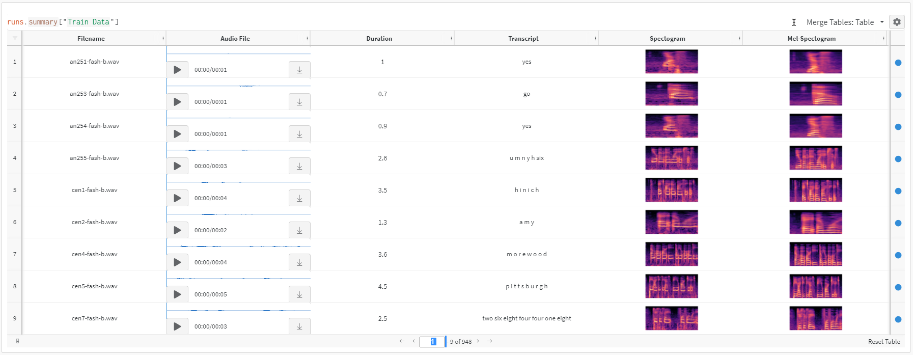
As can be seen, it is much easier to explore the dataset using Weights and Biases tables where everything is one place. You can play the Audio and also check the transcribe.
Great! Now that we've been able to create our own dataset and have a super simple way to explore the data, let's move on.
Specifying Our Model with a YAML Config File
For this tutorial, we'll build a Jasper_4x1 model, with K=4 blocks of single (R=1) sub-blocks and a greedy CTC decoder, using the configuration found in ./configs/config.yaml.
If we open up this config file, we find model section which describes architecture of our model. A model contains an entry labeled encoder, with a field called jasper that contains a list with multiple entries. Each of the members in this list specifies one block in our model, and looks something like this:
- filters: 128repeat: 1kernel: [11]stride: [2]dilation: [1]dropout: 0.2residual: falseseparable: truese: truese_context_size: -1
The first member of the list corresponds to the first block in the Jasper architecture diagram, which appears regardless of K and R.
Next, we have four entries that correspond to the K=4 blocks, and each has repeat: 1 since we are using R=1. These are followed by two more entries for the blocks that appear at the end of our Jasper model before the CTC loss.
There are also some entries at the top of the file that specify how we will handle training (train_ds) and validation (validation_ds) data.
Using a YAML config such as this is helpful for getting a quick and human-readable overview of what your architecture looks like, and allows you to swap out model and run configurations easily without needing to change your code.
It is really difficult to look at the params above. Especially difficult to share params and results with a fellow teammate. Below, we will see how easy it is to use Weights and Biases integration with PyTorch lightning and how Weights and Biases stores results, configs, tables all in one place which is really convenient when trying to replicate results!
Training with PyTorch Lightning & Weights and Biases integration
NeMo models and modules can be used in any PyTorch code where torch.nn.Module is expected.
However, NeMo's models are based on Pytorch Lightning's LightningModule and we recommend you use Lightning for training and fine-tuning as it makes using mixed precision and distributed training very easy. So to start, let's create Trainer instance for training on GPU for 50 epochs.
import pytorch_lightning as pltrainer = pl.Trainer(gpus=1, max_epochs=50)
Did you know that Weights and Biases has already been integrated into popular frameworks such as PyTorch Lightning? We could at this stage just use a WandbLogger to log all our progress during training to Weights and Biases!
import pytorch_lightning as plfrom pytorch_lightning.loggers import WandbLogger# initialize W&B logger and specify project name to store results towandb_logger = WandbLogger(project="ASR", log_model='all')# set config params for W&B experimentfor k,v in params.items():wandb_logger.experiment.config[k]=v# initialize trainer with W&B loggertrainer = pl.Trainer(gpus=1, max_epochs=10, logger=wandb_logger)
This is great because it allows us to replicate experiments very easily.
Next, we instantiate and ASR model based on our config.yaml file from the previous section. Note that this is a stage during which we also tell the model where our training and validation manifests are.
# Update train and test data pathparams['model']['train_ds']['manifest_filepath'] = train_manifestparams['model']['validation_ds']['manifest_filepath'] = test_manifest# initialize modelfirst_asr_model = nemo_asr.models.EncDecCTCModel(cfg=DictConfig(params['model']), trainer=trainer)
With that, we can start training with just one line!
# Start training - this will automatically store results to Weights and Biasestrainer.fit(first_asr_model)wandb.finish();
There we go! We've put together a full training pipeline for the model and trained it for 10 epochs.
Weights and Biases: Hyperparameter tuning using Sweeps
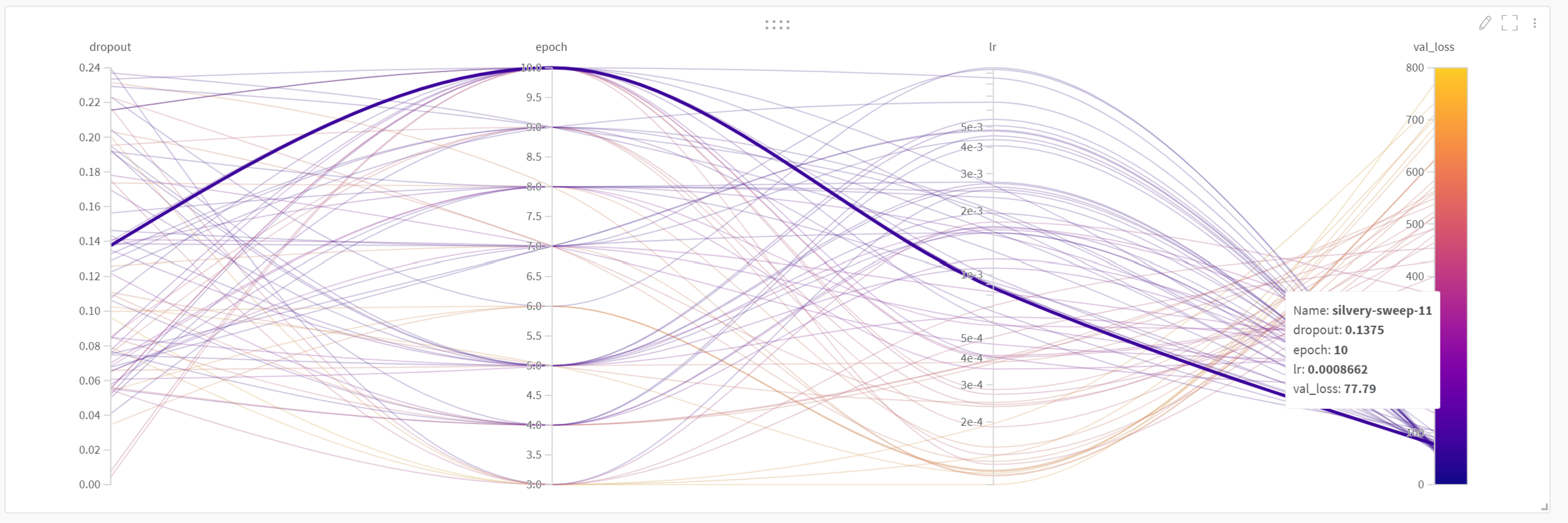
Additionally we might also want to tune some hyperparameters. Below, I've just taken a small subset of all the possible parameters in params, such as lr, epoch and dropout to showcase hyperparameter tuning using W&B Sweeps.
There are many benefits of using W&B sweeps, from the docs:
- Quick setup: Get going with just a few lines of code. You can launch a sweep across dozens of machines, and it's just as easy as starting a sweep on your laptop.
- Transparent: We cite all the algorithms we're using, and our code is open source.
- Powerful: Our sweeps are completely customizable and configurable.
It's really simple to add sweeps to this ASR example. First, we define a sweep config as below:
sweep_config = {"method": "random", # Random search"metric": { # We want to minimize `val_loss`"name": "val_loss","goal": "minimize"},"parameters": {"lr": {# log uniform distribution between exp(min) and exp(max)"distribution": "log_uniform","min": -9.21, # exp(-9.21) = 1e-4"max": -4.61 # exp(-4.61) = 1e-2},"epoch": {"distribution": "int_uniform","min": 3,"max": 10},"dropout": {"distribution": "uniform","min": 0,"max": 0.25}}}
Next, we define a sweep_iteration function as below. The key difference is that now the values of these are taken from wandb.config instead of being set to hard values.
Example,
params['model']['optim']['lr'] = wandb.config.lrparams['model']['encoder']['jasper'][-1]['dropout'] = wandb.config.dropout
Because these values change with every sweep, we take these values from wandb.config as below.
def sweep_iteration():# load configconfig_path = './configs/config.yaml'yaml = YAML(typ='safe')with open(config_path) as f:params = yaml.load(f)# set up W&B loggerwandb.init() # required to have access to `wandb.config`wandb_logger = WandbLogger(log_model='all') # log final model# setup dataparams['model']['train_ds']['manifest_filepath'] = train_manifestparams['model']['validation_ds']['manifest_filepath'] = test_manifest# setup sweep paramparams['model']['optim']['lr'] = wandb.config.lrparams['model']['encoder']['jasper'][-1]['dropout'] = wandb.config.dropouttrainer = pl.Trainer(gpus=1, max_epochs=wandb.config.epoch, logger=wandb_logger)# setup model - note how we refer to sweep parameters with wandb.configmodel = nemo_asr.models.EncDecCTCModel(cfg=DictConfig(params['model']), trainer=trainer)# traintrainer.fit(model)
Finally, we create a wandb sweep and pass in the wandb_config to it. Next, we simply create an agent that runs various runs and based on the sweep "method", selects parameters to compare val_loss for various parameter values.
sweep_id = wandb.sweep(sweep_config, project="ASR")wandb.agent(sweep_id, function=sweep_iteration)
You can see the results of running this sweep here. As you can see we get this beautiful plot as below from which it is much easier to how various hyperparameter lead to validation loss values.
Weights and Biases: Log performance metrics
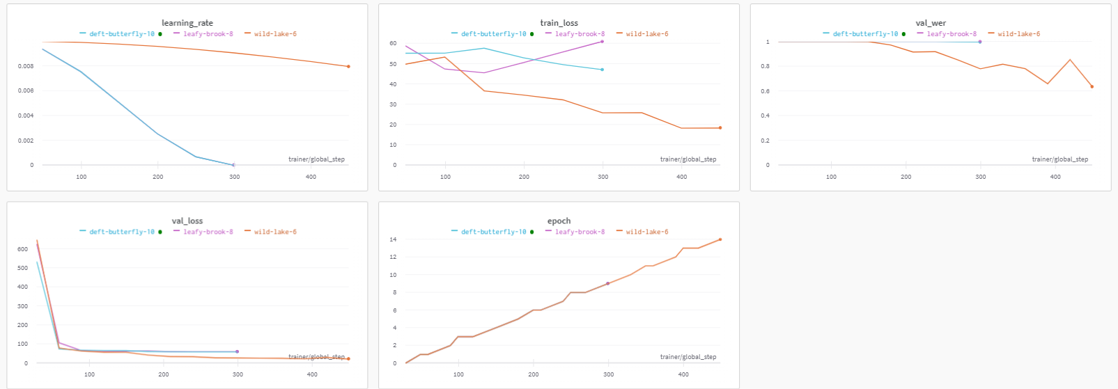
Running the above training code also stores all training metrics to W&B and creates an easy to read Dashboard. You can find the logged training metrics at the Dashboard here.
This dashboard looks like below:

As can be seen in the dashboard above, it is super easy to see learning rate, train loss and validation loss metrics which wouldn't have been possible without logging metrics to Weights and Biases.
Weights and Biases: Log Config
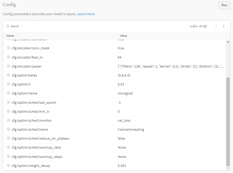
Another benefit that we get from storing results to Weights and Biases is the config params, it is much easier and simpler to look at the parameters as shown below:
Weights and Biases: Compare Experiments
Logging to W&B also makes it super simple to compare experiments. You can find the example of ASR experiments here.
Weights and Biases: Model Artifacts
If you'd like to save this model checkpoint for loading later (e.g. for fine-tuning, or for continuing training), you can simply call first_asr_model.save_to(<checkpoint_path>). Then, to restore your weights, you can rebuild the model using the config (let's say you call it first_asr_model_continued this time) and call first_asr_model_continued.restore_from(<checkpoint_path>).
Another quick way to save progress and model weights is to use Weights and Biases artifacts. Since we passed log_model='all' to WandbLogger, Weights and Biases has already stored all model weights after every epoch.

It is really simple to use any of these model weights! All we need to do is run the following 2 lines of code:
artifact = run.use_artifact('user_name/project_name/new_artifact:v1', type='my_dataset')artifact_dir = artifact.download()
As can be seen, this downloads the model to './artifacts/model-2kr60tp1:v9'
Inference
Let's have a quick look at how one could run inference with NeMo's ASR model.
First, EncDecCTCModel and its subclasses contain a handy transcribe method which can be used to simply obtain audio files' transcriptions. It also has batch_size argument to improve performance.
if LOG_WANDB:preds = quartznet.transcribe(paths2audio_files=test_audio_paths, batch_size=16)pred_table = wandb.Table(columns=['FileName', 'Audio', 'Prediction', 'Ground Truth'])for path, gt, pred in zip(test_audio_paths, test_texts, preds):pred_table.add_data(os.path.basename(path), wandb.Audio(path), pred, gt)run = wandb.init(project='ASR')wandb.log({'Prediction Table': pred_table})wandb.finish();
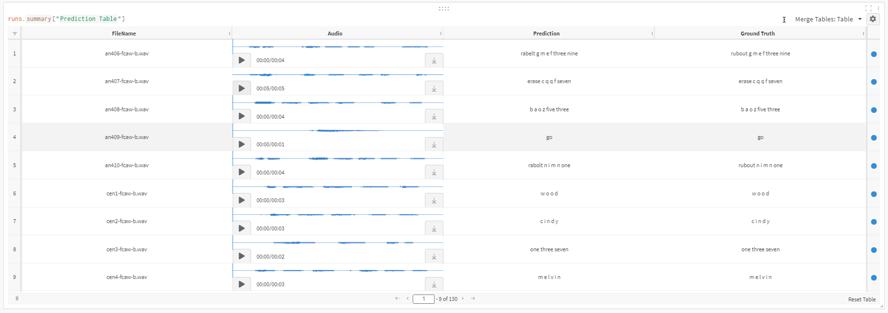
You can find the same interactive table here. It is really easy now to compare and look at predictions from our model.
Also, below is an example of a simple inference loop in pure PyTorch. It also shows how one can compute Word Error Rate (WER) metric between predictions and references.
import copynew_opt = copy.deepcopy(params['model']['optim'])new_opt['lr'] = 0.001first_asr_model.setup_optimization(optim_config=DictConfig(new_opt))# Bigger batch-size = bigger throughputparams['model']['validation_ds']['batch_size'] = 16# Setup the test data loader and make sure the model is on GPUfirst_asr_model.setup_test_data(test_data_config=params['model']['validation_ds'])first_asr_model.cuda()# We will be computing Word Error Rate (WER) metric between our hypothesis and predictions.# WER is computed as numerator/denominator.# We'll gather all the test batches' numerators and denominators.wer_nums = []wer_denoms = []# Loop over all test batches.# Iterating over the model's `test_dataloader` will give us:# (audio_signal, audio_signal_length, transcript_tokens, transcript_length)# See the AudioToCharDataset for more details.for test_batch in first_asr_model.test_dataloader():test_batch = [x.cuda() for x in test_batch]targets = test_batch[2]targets_lengths = test_batch[3]log_probs, encoded_len, greedy_predictions = first_asr_model(input_signal=test_batch[0], input_signal_length=test_batch[1])# Notice the model has a helper object to compute WERfirst_asr_model._wer.update(greedy_predictions, targets, targets_lengths)_, wer_num, wer_denom = first_asr_model._wer.compute()first_asr_model._wer.reset()wer_nums.append(wer_num.detach().cpu().numpy())wer_denoms.append(wer_denom.detach().cpu().numpy())# Release tensors from GPU memorydel test_batch, log_probs, targets, targets_lengths, encoded_len, greedy_predictions# We need to sum all numerators and denominators first. Then divide.print(f"WER = {sum(wer_nums)/sum(wer_denoms)}")
This WER is not particularly impressive and could be significantly improved. You could train longer (try 100 epochs) to get a better number. Check out the next section on how to improve it further.
Model Improvements
You already have all you need to create your own ASR model in NeMo, but there are a few more tricks that you can employ if you so desire. In this section, we'll briefly cover a few possibilities for improving an ASR model.
Data Augmentation
There exist several ASR data augmentation methods that can increase the size of our training set.
For example, we can perform augmentation on the spectrograms by zeroing out specific frequency segments ("frequency masking") or time segments ("time masking") as described by SpecAugment, or zero out rectangles on the spectrogram as in Cutout. In NeMo, we can do all three of these by simply adding in a SpectrogramAugmentation neural module.
Transfer Learning
Transfer learning is an important machine learning technique that uses a model’s knowledge of one task to make it perform better on another. Fine-tuning is one of the techniques to perform transfer learning. It is an essential part of the recipe for many state-of-the-art results where a base model is first pretrained on a task with abundant training data and then fine-tuned on different tasks of interest where the training data is less abundant or even scarce.
In ASR you might want to do fine-tuning in multiple scenarios, for example, when you want to improve your model's performance on a particular domain (medical, financial, etc.) or on accented speech. You can even transfer learn from one language to another! Check out this paper for examples.
Transfer learning with NeMo is simple. Let's demonstrate how the model we got from the cloud could be fine-tuned on AN4 data. (NOTE: this is a toy example). And, while we are at it, we will change model's vocabulary, just to demonstrate how it's done.
# Check what kind of vocabulary/alphabet the model has right nowprint(quartznet.decoder.vocabulary)# Let's add "!" symbol there. Note that you can (and should!) change the vocabulary# entirely when fine-tuning using a different language.quartznet.change_vocabulary(new_vocabulary=[' ', 'a', 'b', 'c', 'd', 'e', 'f', 'g', 'h', 'i', 'j', 'k', 'l', 'm', 'n','o', 'p', 'q', 'r', 's', 't', 'u', 'v', 'w', 'x', 'y', 'z', "'", "!"])>> [' ', 'a', 'b', 'c', 'd', 'e', 'f', 'g', 'h', 'i', 'j', 'k', 'l', 'm', 'n', 'o', 'p', 'q', 'r', 's', 't', 'u', 'v', 'w', 'x', 'y', 'z', "'"][NeMo I 2022-01-19 15:31:05 ctc_models:348] Changed decoder to output to [' ', 'a', 'b', 'c', 'd', 'e', 'f', 'g', 'h', 'i', 'j', 'k', 'l', 'm', 'n', 'o', 'p', 'q', 'r', 's', 't', 'u', 'v', 'w', 'x', 'y', 'z', "'", '!'] vocabulary.
After this, our decoder has completely changed, but our encoder (which is where most of the weights are) remained intact. Let's fine tune-this model for 2 epochs on AN4 dataset.
# Use the smaller learning rate we set beforequartznet.setup_optimization(optim_config=DictConfig(new_opt))# Point to the data we'll use for fine-tuning as the training setquartznet.setup_training_data(train_data_config=params['model']['train_ds'])# Point to the new validation data for fine-tuningquartznet.setup_validation_data(val_data_config=params['model']['validation_ds'])# And now we can create a PyTorch Lightning trainer and call `fit` again.trainer = pl.Trainer(gpus=[1], max_epochs=2)
Further Reading/Watching:
That's all for now! If you'd like to learn more about the topics covered in this tutorial, here are some resources that may interest you:
Add a comment
Iterate on AI agents and models faster. Try Weights & Biases today.
